Work and Span

By Aditi Gupta and Brandon Wu, May 2020. Revised December 2022

We will now turn towards a more robust notion of work and span that let us analyze our conception of asymptotic runtime more effectively. It is still dependent on asymptotic analysis, but merely involves being more involved with how we go about generating the asymptotic bound for a function from the code itself. Additionally, we will not only analyze the approximate number of steps of the program (which corresponds to the runtime of the program, given sequential execution), but also the approximate longest chain of dependencies that exists in the program, assuming that computations can be run in parallel. We will elaborate more on this idea in this chapter.

Parallel Computing

It is intuitive to view things occurring sequentially. Whether it is reading a tutorial, writing a list of instructions, or making a plan for the future, sequential actions are very easy to think about. Even programs are written in a stepwise manner, with computations happening one after the other in a prescribed way. It seems to be in our nature to impose some kind of order on a list of actions.

Despite that, however, sequential evaluation is not always the most efficient. Sequential evaluation introduces dependencies where other subtasks cannot be started until we have finished the current subtask, which has the effect of potentially inducing wait times where none exist. For instance, if your plan is to do the laundry and your homework, it might not be the most time-efficient to wait until the washer is done before get started on your work. There is no dependency between laundry and homework - there is no logical reason why you should have to wait for one before the other, so you could do them both at the same time, or in parallel.

Parallel computing is a principle that is becoming more and more important as time goes on. Computers now more frequently have multiple cores in their processors, which means that tasks can be subdivided and assigned out to independent acting agents.

The benefits of doing so are clear. Suppose that we are stacking a shelf with merchandise. If the shelf is tall, this may take us a while - roughly linear in the height of the shelf, we can imagine (supposing we have an infinite stock of items, and that climbing a ladder somehow isn't a factor). If we had a person to dedicate to each shelf, however, then we could stock the shelves in "constant" time - independent of the number of shelves that there actually are. This will be a driving idea behind how we look at parallelism.

While we will not delve into the implementation details of parallel computing (which is more apt for a systems perspective), we will perform basic analysis of asymptotic complexity based on that premise. These take the form of work and span, fundamental ideas that will drive the next section.

Theory

First, let us consider what we will term a task dependency graph. This is not so important of a concept to memorize, but it will help in conceptualizing work and span. A task dependency graph is a directed acyclic graph (that is, a graph whose edges are one-way, and there exist no loops) that represents the dependencies when trying to perform a set of tasks. Each node is a task, labelled with the time that it takes to execute it (which is a singular unit, unable to be reduced otherwise), as well as edges that represent the dependencies in the graph. Any task cannot be started until all of the tasks that have edges directed towards it are finished - that is, all of a task's inbound edges denote its prerequisites.

With this knowledge, we will be able to define what we mean by work and span.

[Work] The work of a computation denotes the number of steps it takes to run, assuming access to only a single processor. Work thus represents the worst-case sequential evaluation time, and can be upper bounded with asymptotic analysis.

[Span] The span of a computation denotes the number of steps that it takes to run, assuming access to infinitely many processors that allow us to run tasks in parallel. Span thus represents the worst-case parallel evaluation time, and can be upper bounded with asymptotic analysis.

What we find is that work directly corresponds to our previous intuition of the complexity of a computation, since our previous analyses have always been sequential. Span, however, is not quite as easy to eyeball. Now, we are really looking for the longest chain of dependencies, that is, the longest sequence of tasks that must be run sequentially, since everything else can be run concurrently. Infinitely many processors, while obviously unrealistic, helps to simplify our analysis, and provides us a "target" for the efficiency of a fully parallel algorithm.

We illustrate these concepts with the following graph.

Fig 1. Task dependency graph illustrating dependencies between tasks and task durations

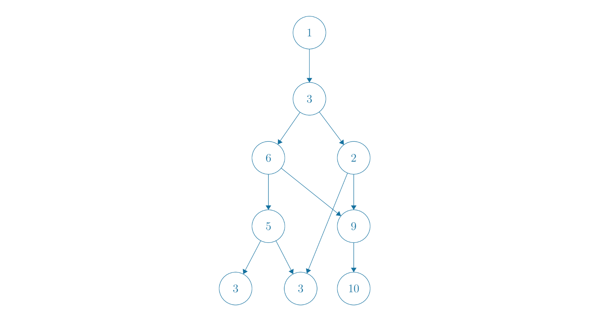
So in this example, the work of our graph would be $1+3+6+2+5+9+3+3+10 = 42$, since with a single processor, the dependencies don't really matter to us. We have no choice but to complete every task, and the precise order doesn't matter. That isn't to say that we can execute the tasks in any order, that plainly isn't true - we simply mean that there is no order that can change what our runtime is.

On the other hand, for span we must consider the length of the longest path. The span of this graph would thus be $1 + 3 + 6 + 9 + 10 = 29$, since that is the longest path. Even being able to execute everything else in a parallel way, we cannot avoid the fact that these nodes must follow one after the other. This path is thus the limiting factor in our runtime - ultimately it constrains the amount of time that we expend.

Task dependency graphs are a concept that we discuss purely for theoretically being able to understand the idea of work and span. We will look at examples in terms of actual SML code in the next section, which will be primarily where we do our work/span analysis.

Work/Span Analysis of Code

The previous example was rather contrived. For one thing, it is prespecified - we already knew all of the tasks that there were, along with its dependencies and task times. As such, we could compute a simple, numerical answer. This will likely not be the case. We are interested in work/span analysis of algorithms, which will yield us another function - one describing the runtime complexity of the algorithm as a function of some notion of input size.

For recursive functions, work/span analysis is very easy to do. We characterize it in terms of recurrence relations, which are themselves recursive functions describing the work or span of some code. Then, we simply solve for the closed form of the recurrence relation and estimate a Big-O bound to arrive at our desired complexity.

Consider the following example:

fun length ([] : int list) : int = 0
  | length (x::xs : int list) : int = 1 + length xs

The first step to determining the work and span of such a function is to write a recurrence relation. These steps are explicit - the code should determine the recurrence relation, and the recurrence relation should determine the Big-O bound. We will first analyze this function's work complexity, then move on to span.

First, we should fix some notion of input size. This will differ based on what our recurrence is recursing on, but in this example it seems to be the size of the input list. Note that this follows directly from the code - if this were the factorial function, we may say that the recurrence is in terms of the value of the input, and as we will later see, if the input was a tree, we may write the recurrence in terms of the number of nodes in the tree.

So we can write the following recurrence for work. We will explain soon what exactly it means, and how to arrive at it:

$$\begin{aligned} W_{length}(0) &= c_1 \\ W_{length}(n) &= c_0 + W_{length}(n-1) \end{aligned}$$

This recurrence is made of two parts - the recursive case and the base case. The first equation for $W_{length}(n)$ simply denotes what the work for an input size of $n$ should be - defined recursively. The second equation for $W_{length}(0)$ defines what the work for an input size of $0$ should be. This directly corresponds to our code, which has two clauses for a list of length $0$ (that being []), and for the general case. This is an important observation to make, that the recurrence follows directly from the code.

The recursive case says that, for an input of size $n$, the work done is $c_0 + W_{length}(n-1)$. Here, $c_0$ denotes some constant. This is supposed to correspond to the recursive case of the function, and if we look at it, we have a recursive call length xs, as well as some other work of adding one. Adding one, being an arithmetic operation, is a constant-time process, meaning that it takes a non-zero constant amount of time. This is what $c_0$ is supposed to represent - the constant amount of non-recursive work that must be done, after the recursive call has finished. It is not important what $c_0$ is, just that it is some unspecified amount of work that is not a function of $n$.

Conversely, $W_{length}(n-1)$ represents exactly the amount of work done by the recursive call, since it is literally defined to be the amount of work done by an input of size $n-1$, which is exactly what happens when we call length xs, where xs has length $n-1$.

NOTE: Even if we did not have the addition operation, we would still have $c_0$. This is because merely entering the function and figuring out which case to execute takes some non-zero amount of work - it is impossible to run the recursive call perfectly with no other time expense. As such, we would see exactly the same recurrence even if the recursive case was length (x::xs : int list) : int = length xs (which would also be a very bad length function).

For the base case, we have that $W_{length}(0) = c_1$, since in the base case we just return 0. This has a constant amount of work associated with it, as argued previously, so we use the constant $c_1$ to denote that, since the amount of work is likely not the same constant as that in the recursive case, when adding 1.

So this is how we arrive at the work recurrence for length. We will now turn to the span recurrence, which we obtain as:

$$\begin{aligned} S_{length}(0) &= c_1 \\ S_{length}(n) &= c_0 + S_{length}(n-1) \end{aligned}$$

Note that the span recurrence is exactly the same as the work recurrence. This should make sense, because there is no opportunity for parallelism in the length function - we can only pop off elements one by one from the list. In the recursive case, we must wait for the result of the recursive call on xs, which means we unavoidably must expend the span of $S_{length}(n-1)$ - additionally, we have a data dependency. We cannot execute the addition in 1 + length xs until we obtain the result for length xs, which means that we must sum the time it takes to compute length xs (that being $S_{length}(n-1)$) and the time it takes to carry out the addition operation (that being $c_1$).

Now we will begin the task of actually solving the recurrence. They are the same recurrence, so without loss of generality we will solve just the work recurrence.

We know that it has the form of $W_{length}(n) = c_0 + W_{length}(n-1)$, and eventually reaches a base case at $W_{length}(0) = c_1$. We can "unroll" the recurrence a few times to see if we can see a pattern, and then arrive at our answer.

So we start out with $W_{length}(n) = c_0 + W_{length}(n-1)$, but if we invoke the definition of $W_{length}(n-1)$, we can produce $c_0 + c_0 + W_{length}(n-2)$, since $W_{length}(n-1) = c_0 + W_{length}(n-2)$. By doing the same for $W_{length}(n-2)$, we get $c_0 + c_0 + c_0 + W_{length}(n-3)$. It seems we've hit upon a pattern - each time we "unroll" the definition of $W_{length}(n)$, for progressively lower $n$, we get another $c_0$ term back out. Then, we know that the recurrence should eventually solve to:

$$W_{length}(n) = (\sum_{i = 1}^n c_0) + c_1$$

We will usually omit the $c_1$, since it does not matter asymptotically. Then, clearly this is equivalent to $nc_0 + c_1$. We see that this closed-form solution is linear in $n$ - so then we have that the work and span of this function is in $O(n)$, which is consistent with what we would expect if we had "eyeballed" it.

Work/Span Analysis: Trees

First, we will discuss the definition of a binary tree in SML:

datatype tree = Empty | Node of tree * int * tree

This denotes that a tree is either the constant constructor Empty denoting the empty tree, or a Node that contains an integer value, as well as two tree children, that can themselves be Nodes or Empty.

Fig 2. Sample binary tree

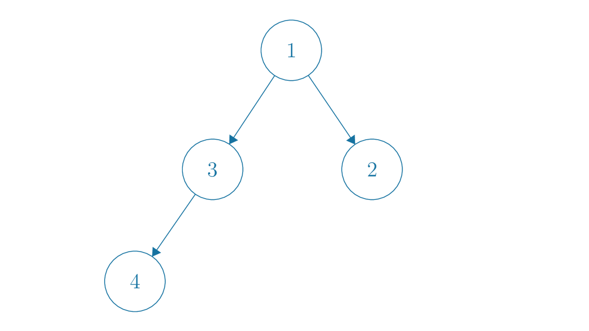
So for instance, we may represent the above tree with Node(Node(Node(Empty, 4, Empty), 3, Empty), 1, Node(Empty, 2, Empty)). Put more fancily:

Node(
    Node(
        Node(
            Empty,
            4,
            Empty
        ),
        3,
        Empty
    ),
    1,
    Node(
        Empty,
        2,
        Empty
    )
)

Now we will analyze the complexity of finding the size of a tree. Consider the following implementation for doing so:

fun size (Empty : tree) : int = 0
  | size (Node (L,x,R) : tree) : int = size L + 1 + size R

First convince yourself that it actually works. It simply recursively finds the size of the left and right tree, then adds one for the node that it is currently at. In the empty case, we consider the empty tree to have a size of 0.

The major difference between this function and the previous length function was that length had one recursive call - size has two. We will need to reflect this change when we write our recurrences. Additionally, we need a new variable for our recurrence - we no longer have a list whose length we can induct on. A similar analogue will be $n$, the number of nodes in the tree, so we will take that as our recurrence variable. We will focus first on work.

We will obtain the following work recurrence:

$$\begin{aligned} W_{size}(0) &= c_1 \\ W_{size}(n) &= c_0 + W_{size}(n_l) + W_{size}(n_r) \end{aligned}$$

where we define the number of nodes in the tree $n = 1 + n_l + n_r$, and $n_l$ and $n_r$ denote the number of nodes in the left and right subtree, respectively. This follows similarly to our recurrence for length in the previous part, where c_0 is just some constant amount of work that we necessarily have to do, and the two $W_{size}$ calls are from the two recursive calls we make to L and R.

Now, we don't know precisely how big $n_l$ and $n_r$ are, with respect to $n$. This makes our analysis a little more tricky, but essentially all we need to do is think of the worst case, as we are interested in the worst-case asymptotic complexity of this function. For work, however, there is no worst-case - no matter how the tree is structured, we must visit every node once, doing a constant amount of work each time. So we should obtain, in the end, $W_{size}(n) = nc_0 + c_1$, which we know is $O(n)$. So in this case, we didn't have to think about the structure of the tree. In the next section, it will matter.

Work/Span Analysis: Balanced vs Unbalanced Trees

We will revisit the same example, except from the perspective of span.

The important point to note is that, now, we have two separate recursive calls that are happening in the recursive call of size. These recursive calls have no data dependency - neither running depends on the other. This means that they can be run in parallel, which means that the total span that we compute should just be the max over both. This is because we can imagine that both of them lead to different "paths" in our task-dependency graph - we are only interested in the maximum-length path. So we will run both results, and whichever one takes longer to return an answer to us is the "limiting reagent" of our computation.

So we will write the span recurrence as follows:

$$\begin{aligned} S_{size}(0) &= c_1 \\ S_{size}(n) &= c_0 + \max(S_{size}(n_l), S_{size}(n_r)) \end{aligned}$$

Now note that we are taking the max over the two recursive calls. Now, we cannot handwave the structure of the tree like we did in the previous part - if one path is significantly longer than the other, then it will stall the computation for longer. We still must visit every node, but some of them can occur in parallel.

We will consider the first case - if we have an unbalanced tree. Suppose that the tree is heavily unbalanced - akin to a (diagonal) linked list. Without loss of generality, let it be "pointing" to the left. Then, $n_l = n - 1$, and $n_r = 0$. Then, the max over both recursive calls should clearly be that of $S_{size}(n-1)$, since it has to compute the size of a larger tree.

So we can update our recurrence and obtain:

$$\begin{aligned} S_{size}(0) &= c_1 \\ S_{size}(n) &= c_0 + S_{size}(n-1) \end{aligned}$$

This recurrence is exactly the same as that of length, so we know that we will get that $S(n) \in O(n)$. This should make sense intuitively, since the depth of the tree is $n$, and there are dependencies between each level - we cannot go to the next level until we are done with the current one. So we cannot avoid having to visit every level sequentially, which results in $O(n)$ span.

Now, what if we consider a balanced tree? Well, the balanced case would be if the number of nodes in the left and right subtrees are roughly equal - that is, $n_l = n_r = \frac{n}{2}$. We will consider them exactly equal to simplify our analysis, but we will obtain the same asymptotic answer. Then, we know that the maximum is just any one of them, since they will have the same span.

So we can update our recurrence and obtain:

$$\begin{aligned} S_{size}(0) &= c_1 \\ S_{size}(n) &= c_0 + S_{size}(\frac{n}{2}) \end{aligned}$$

This is slightly different than our length recurrence. We will try unrolling to make sense of this recurrence.

We have that $S_{size}(n) = c_0 + S_{size}(\frac{n}{2})$. Plugging in the recursive definition of $S_{size}(\frac{n}{2})$, we get that this expands to $c_0 + c_0 + S_{size}(\frac{n}{4})$, which by the same trick expands to $c_0+ c_0 + c_0 + S_{size}(\frac{n}{8})$, and so on and so forth. We note that we are dividing the number of nodes by 2 each time - and we know that we can divide $n$ by two roughly $\log_2(n)$ times. So in total, we can solve the summation of $S_{size}(n)$ as $S_{size}(n) = (\sum_{i=1}^{\log_2(n)} c_0) + c_1$.

So then this simplifies to $S_{size}(n) = \log_2(n)c_0 + c_1$. This is a logarithmic function of $n$, so we get that the span of size is in $O(\log n)$. Thus, we obtain a different span for balanced trees versus unbalanced trees - balanced trees are more efficient and parallelism-friendly.

Work/Span Analysis: Size-dependent Operations

In these past two examples, we have only seen examples that did a constant amount of non-recursive work. We will now analyze a function that does non-recursive work that is a function of the input size $n$. This will result in different kinds of recurrences. First, however, we will digress briefly to motivate the example that we will analyze.

[Case Study: Tree Traversal]

When analyzing trees, it is often prudent to utilize tree traversal, or a systematic way of enumerating the elements in a tree. There are multiple different ways to do this, depending on what your intentions are - a few namely being preorder, inorder, and postorder traversal.

With these different methods of traversal, we can turn a tree into a different kind of ordered data structure, such as a list or sequence. This can come in handy when we desire future fast access to any arbitrarily ranked node in the tree, or if we want to convert it for purposes of printing, for instance.

Each traversal is characterized by a certain "strategy" of traversal, depending on how it ranks the three possible directions that it can go - root, left, and right. Inorder traversal, for instance, is characterized by left-root-right prioritization - this means that it goes left first, and if it can't go left, then it visits the root node, and otherwise it goes right. Note that this does not mean that it visits the root of the left subtree first - it simply reruns the same process on the entire left subtree. No matter what the traversal strategy is, a node is never actually visited until the "root" action is taken. Preorder traversal is root-left-right, and postorder is left-right-root. Examples of preorder and inorder traversals (the most common you will see in this book) are below.

Fig 3. An example of a preorder traversal (left) and inorder traversal (right) of a binary tree, with visited nodes labeled in ascending order

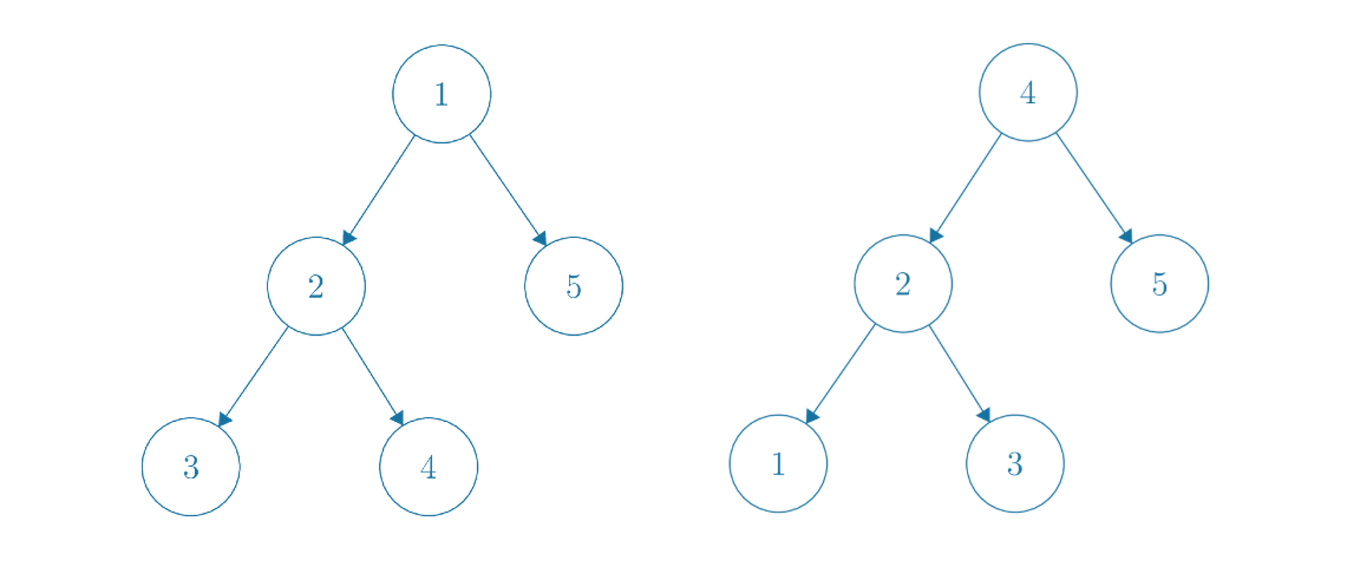
Tree traversals can also come in handy when generating different notations for mathematical expressions when represented in the form of an binary expression tree, which has nodes that consist of either a numeric constant, which has no children, a unary operation with a single child, or a binary operation with two children. For instance, a binary expression tree for the mathematical expression $(4-1) * 2$ is shown below.

Fig 4. A binary expression tree for the expression (4 - 1) * 2

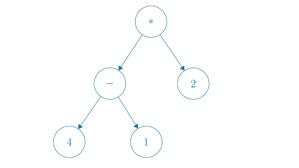
With inorder traversal of this expression tree, we can generate the constants and symbols in exactly the same order as $(4-1) * 2$, which is how we would normally interpret it. Preorder and postorder traversal, however, result in an interesting interpretation - what is known as prefix (or Polish) and postfix (or Reverse Polish) notation.

In prefix notation, by using preorder traversal, we obtain the expression * - 4 1 2, which is how we would interpret the same expression if all of our operators appeared before their operands. Similarly, with postorder traversal, we obtain the expression 4 1 - 2 * in postfix notation. Prefix and postfix notation have significance in their lack of ambiguity - while infix notation is easy for humans to read, it requires parentheses sometimes to denote how operator precedence takes place. Prefix and postfix notation have no such flaw - they are unambiguous in how operations take place. In programming language interpreters, such notations are sometimes used to represent mathematical expressions.

Such a digression serves as motivation for the next function that we will analyze - which is writing the preorder traversal of a tree in SML. The code looks like this:

fun preord (Empty : tree) : int list = []
  | preord (Node(L, x, R) : tree) : int list = x :: (preord L @ preord R)

We can readily see that this follows the root-left-right order that we specified earlier for preorder traversal. Recall that @ is the function for list concatenation, and has a complexity of $O(n_l)$ in $n_l$, the size of the left input list. Thus, as stated before, this function has a non-constant amount of work at each recursive call - we must evaluate @ of the result of preord L and preord R, which is a function of $n$, the number of nodes in the tree.

We will analyze only the balanced case for this function. We invite the reader to think about the unbalanced case on their own.

For the recursive case, we know that $W_{preord}(n)$ will take the form of $c_0 + W_@(n_l) + W_{preord}(n_l) + W_{preord}(n_r)$. By our balanced assumption, we know $n_l = n_r = \frac{n}{2}$, so we can write our work recurrence as:

$$\begin{aligned} W_{preord}(0) &= c_2 \\ W_{preord}(n) &= c_0 + \frac{n}{2}c_1 + 2W_{preord}(\frac{n}{2}) \end{aligned}$$

Note that the term $W_@(n_l)$ is a recurrence in terms of $n$, the size of the left list given as input to @. Since we know that the work complexity of @ is $O(n)$, we can replace $W_@(\frac{n}{2})$ with $\frac{n}{2}c_1$, which is simply some constant $c_1$, scaled by a linear factor of the input $\frac{n}{2}$. This is how we will generally deal with analyzing the complexity of functions that make use of helper functions.

We will make use of a new method to solve this recurrence - the Tree Method.

[Tree Method] The tree method is a method for solving recurrences of certain recurrences that sum to the same quantity across levels, and usually have multiple recursive calls. In essence, if each level has the same amount of computation, then the recurrence solves to the (number of levels) * (amount at each level).

The below diagram illustrates the Tree Method.

Fig 5. An illustration of the Tree Method for the recurrence of preord.

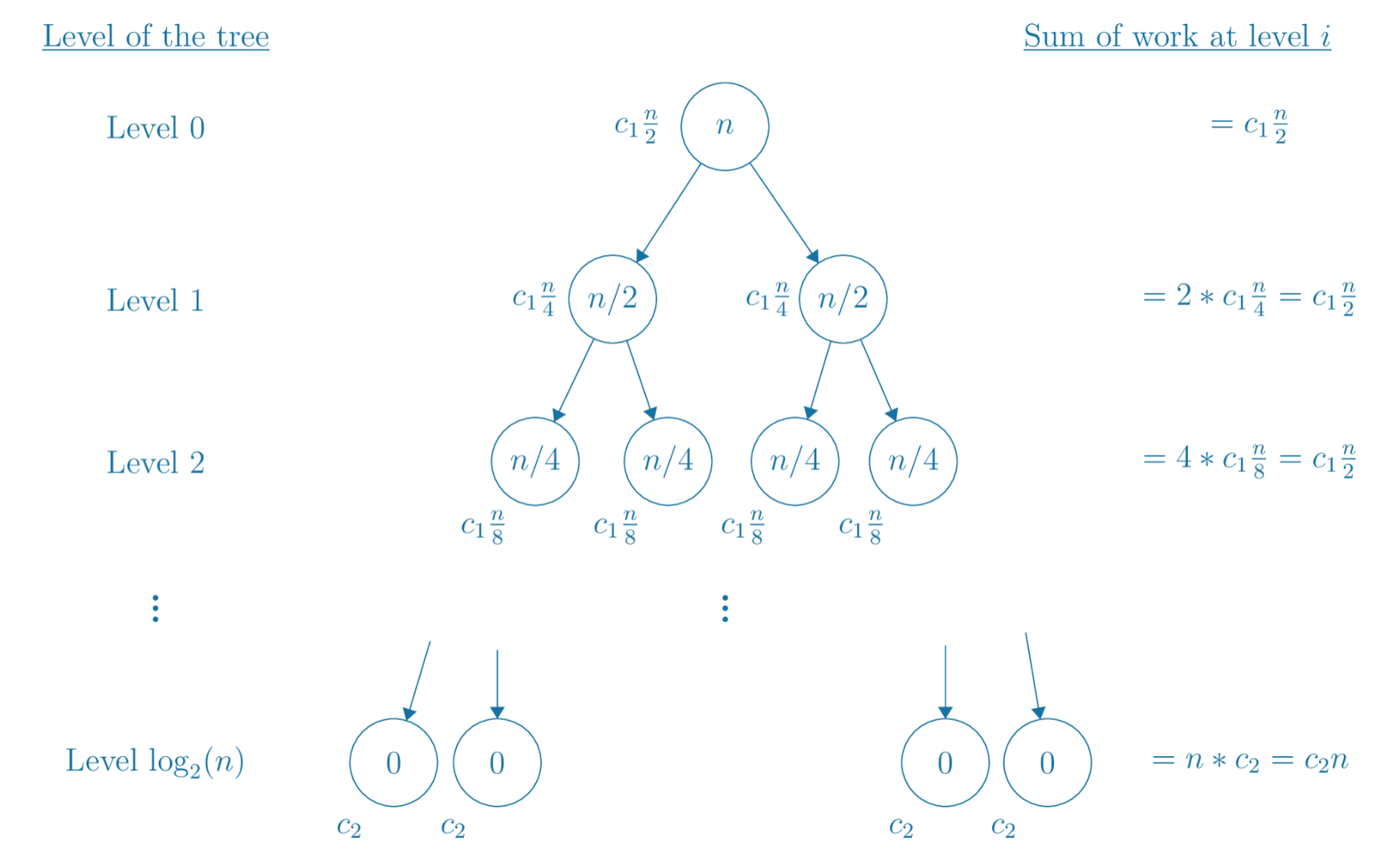
We will now explore exactly how we arrived at this conclusion.

First, note that this tree exists as a result of the recurrence. We used the code to specify the recurrence, and then the recurrence itself described this tree. It has a branching factor of 2 (that is, two children of each node that are non-leaves) since the recursive case of the recurrence has two recursive calls, and at each level the size of the input changes. Since the recursive calls are called on inputs of size $\frac{n}{2}$, each level results in a division by two of the input size.

Additionally, we know that the amount of work at each node (of input size $n$) is necessarily $c_1 \frac{n}{2}$. There is technically also a $c_0$ term, but we will omit it since it is asymptotically dominated by $c_1 \frac{n}{2}$. The precise non-recursive work done by each "node" is specified slightly down and to the left of each node. Individually, they don't look very nice to sum over - at level $i$, it appears the work at each node is $c_1 \frac{n}{2^{i+1}}$. However, level $i$ also has $2^i$ nodes, by the branching nature of the recurrence tree. As such, the total amount of work done at level $i$ is just $c_1 \frac{n}{2^{i+1}} * 2^i = c_1 \frac{n}{2}$, which is not a function of the level $i$.

As such, each level has the same amount of work - which is very convenient, as we can now just take that quantity and multiply it by the number of levels. So in total, when we solve out the recurrence, we should obtain that $W(n) = (\sum_{i=1}^{\log_2(n)} c_1\frac{n}{2}) + c_2n$, since the $c_2n$ term is separately obtained from the base level, due to the $n$ leaves that each have $c_2$ work.

The term $\sum_{i=1}^{\log_2(n)} c_1\frac{n}{2}$ thus goes to $\frac{c_1}{2} n\log_2(n)$, so in total we obtain that $W(n) = \frac{c_1}{2} n\log_2(n) + c_2n$, which is in $O(n \log n)$. So we're done.

The tree method is really nothing more than just a visual way to view the recurrence - it is possible to achieve the same effect by just writing a summation. It is sometimes more intuitive to try and visualize, however, and for recurrences where the levels sum to the same amount, the tree method is very effective. However, not all recurrences exhibit such behavior, and it's hard to know a priori whether a given recurrence is such a one. Nevertheless, it is a powerful method and sufficient for many purposes.

We omit the span analysis of this function for the reader.

Conclusions

Asymptotic analysis is a very important technique for attempting to categorize the efficiency of programs. Moreover, it is not enough to simply find the asymptotic sequential complexity of a function - parallel computation is becoming increasingly more important, and purely sequential analyses are not representative of real-world algorithms. Work and span analyzed through recurrence relations form a powerful framework for examining the complexity of recursive functions, which is robust enough to classify many kinds of algorithms.